Projection and large documents: what MongoDB still reads, measured

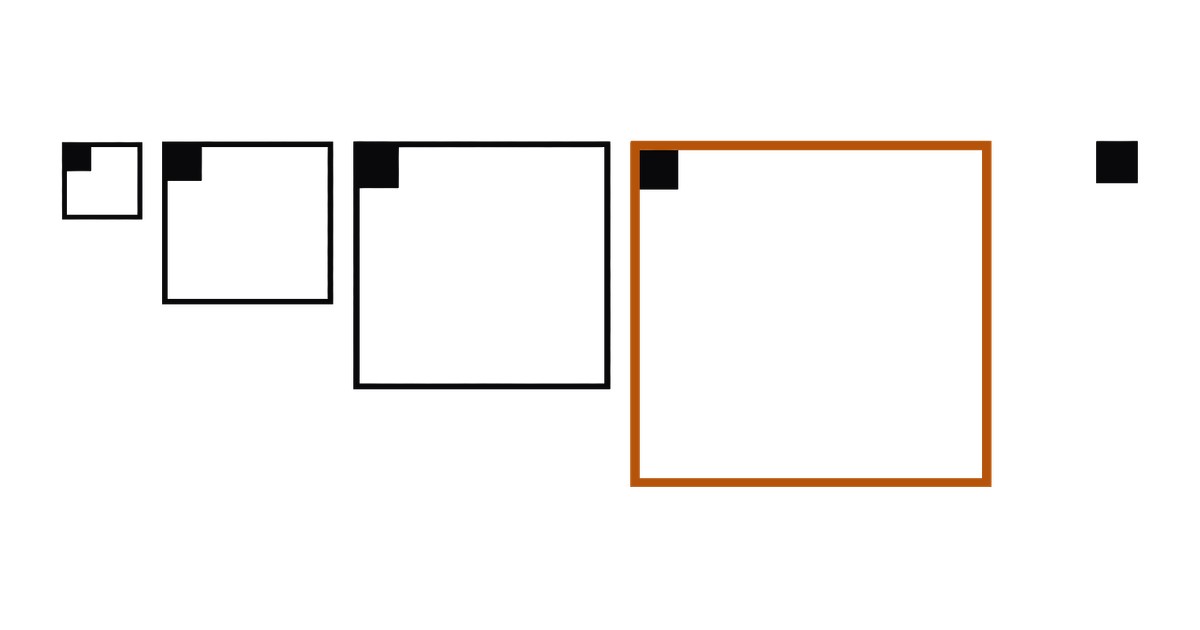
The usual advice about reads is to project only the fields you need. So a list screen that shows the date and the total of each order asks for those two fields and nothing else:

db.orders.find(
  { createdAt: { $gte: from, $lt: to } },
  { createdAt: 1, total: 1 }
)

Over time the orders grow. A history array collects every status change, every note from support and every courier scan, and a document that was 1 KB becomes 64 KB. The query still asks for the same two fields. Does it still cost the same?

I expected it to cost more at every size, because the server has to fetch the document to read the fields out of it. So I measured it, and the first part of that expectation was wrong.

With every document in the cache, the projection cost the same 3 ms on 1 KB documents as on 64 KB ones. The size started to count when the documents no longer fit in the cache. Then the projected query read the whole document from disk to return two fields of it: 61 MB per query to return 48 KB. A covered query, which reads the same two fields from the index, stayed under 3 ms in every case.

What was measured

Four collections, orders_1k, orders_4k, orders_16k and orders_64k, with 50,000 orders in each. The fields a list screen reads, _id, customerId, status, createdAt and total, come from one seed, so they are identical in all four. The only difference is a history array at the end of each document, which fills it to its size:

Collection	Mean document	Data	On disk
orders_1k	1,037 bytes	52 MB	22 MB
orders_4k	4,105 bytes	205 MB	88 MB
orders_16k	16,403 bytes	820 MB	348 MB
orders_64k	65,876 bytes	3,294 MB	1,347 MB

The notes in history are words from a fixed vocabulary, so they compress about as well as real text: the 64 KB collection takes 1,347 MB on disk against 3,294 MB in memory. A field of one repeated character would compress to almost nothing and hide the cost.

Each collection has one index, { createdAt: 1, total: 1 }. There is one order a minute, so a window of 1,000 minutes holds exactly 1,000 orders. Every query reads one such window, sorted by createdAt, in three ways:

1. Whole documents. No projection.
2. A projection of two fields, { createdAt: 1, total: 1 }. This is the query above. It also returns _id, because a projection includes _id unless it says otherwise.
3. A covered query, { _id: 0, createdAt: 1, total: 1 }. Both fields are in the index and _id is not asked for, so the server can answer from the index alone.

Before timing anything, the runner checks that all three return the same 1,000 dates and totals. Beside each timing it prints the time the server spent, from serverStatus().opLatencies, and the bytes WiredTiger read into its cache while the query ran.

With everything in the cache

The first run used the default cache, 15.7 GB, which holds all four collections. Every run read the same window after five warm-up runs.

Document	Whole documents	Projection, two fields	Covered
1 KB	12 ms	3.5 ms	3.1 ms
4 KB	38 ms	2.9 ms	2.5 ms
16 KB	125 ms	3.1 ms	2.6 ms
64 KB	550 ms	3.4 ms	2.6 ms

The projection did its job. The whole-document query grew with the documents, and at 64 KB it returned 66 MB. The server reported 8.5 ms of its own time for that query. The rest of the 550 ms went to moving 66 MB to the application and decoding it there. The projection returned 48 KB at every size, and its time did not move.

The server’s own time tells the same story:

Document	Whole documents	Projection, two fields	Covered
1 KB	0.9 ms	0.8 ms	0.5 ms
4 KB	1.3 ms	0.7 ms	0.4 ms
16 KB	2.5 ms	0.9 ms	0.4 ms
64 KB	8.5 ms	1.0 ms	0.4 ms

The projected query fetched all 1,000 documents at every size, and the plan says so: IXSCAN > FETCH > PROJECTION_SIMPLE, 1,000 documents examined. Fetching a 64 KB document that is already in the cache cost about as much as fetching a 1 KB one. BSON stores the length of each field, so the server can step over the history array without reading through it. In these documents the two projected fields come before the array. I did not measure fields placed after it.

A second run picked a random window from the whole collection for each query, after 50 random warm-up runs. With the 15.7 GB cache the results were the same: the projection took 2.9 to 3.4 ms at every size.

When the documents do not fit in the cache

Many production servers hold only a part of their data in the cache. So the third run used the same data with a 256 MB cache, in a container limited to 1 GB of memory, which also keeps the operating system’s file cache small. Each query again read a random window, after 50 random warm-up runs.

The 1 KB collection is 52 MB in memory, so it fits. The 64 KB one is 3.3 GB, so less than a tenth of it fits.

Document	Whole documents	Projection, two fields	Covered
1 KB	10 ms	3.1 ms	2.7 ms
4 KB	39 ms	3.5 ms	2.4 ms
16 KB	139 ms	8.0 ms	2.3 ms
64 KB	553 ms	34 ms	2.3 ms

And the bytes WiredTiger read into its cache, per query:

Document	Whole documents	Projection, two fields	Covered
1 KB	256 KB	151 KB	0 KB
4 KB	1.0 MB	610 KB	3 KB
16 KB	11 MB	12 MB	10 KB
64 KB	60 MB	61 MB	13 KB

This is the cost the projection does not remove. To return 48 KB, the projected query on 64 KB documents read 61 MB into the cache, the same as the query that returned whole documents. The server reads a document whole before it picks fields out of it, so a projection changes what leaves the server and does not change what the server reads.

At 64 KB the projection took 34 ms against 3.4 ms with the large cache, ten times as long. It was also the least steady number in this post, because it depends on the disk. Two more runs gave 67 ms, and 63 ms over 60 queries. The bytes read stayed at 61 to 62 MB in all three.

The whole-document query hardly changed, at 553 ms here against 550 ms. Two more runs gave 629 ms and 617 ms. At that size, sending 66 MB costs more than reading it from disk, so the slower read hides behind the transfer.

The covered query read 13 KB or less and took 2.3 to 2.7 ms in every row. The index is 1.7 to 1.8 MB in every collection, because it holds the same keys in all four, so it fits in any cache.

Making the query covered

A covered query is the one way in this test that the document size stopped counting, and it takes two changes to the query above. The index has to hold every field the query filters on and every field it returns. The projection has to leave out _id, unless _id is in the index too:

db.orders.createIndex({ createdAt: 1, total: 1 })

db.orders.find(
  { createdAt: { $gte: from, $lt: to } },
  { _id: 0, createdAt: 1, total: 1 }
)

The plan then shows PROJECTION_COVERED with no FETCH under it, and totalDocsExamined: 0. MongoDB’s query optimization page lists what prevents it. A multikey index cannot cover a query on an array field. An equality match on null cannot be covered. On a sharded collection, the index has to contain the shard key.

It has costs of its own. Every field you add to an index makes the index larger. Every insert and delete updates the index, and so does every update that changes an indexed field. This test did not measure that. A covered index is worth it for a few hot list queries, and the wrong answer for every query in an application.

Where a covered query does not fit, the other answer is to move the large part out. If history is read on one screen and the order list is read on every page load, history can live in its own collection, keyed by the order’s _id. Then the orders a list fetches are small again, and more of them fit in the cache.

Checking your own collection

Compare the collection’s size in memory with the cache. collStats reports size, which is the uncompressed size, and storageSize, which is the size on disk:

db.orders.stats().size                  // bytes in memory, uncompressed
db.serverStatus().wiredTiger.cache['maximum bytes configured']

MongoDB’s WiredTiger page gives the default cache as the larger of 50% of RAM minus 1 GB, or 256 MB. It also says the cache holds collection data uncompressed, so the number to compare is size, and not the size on disk.

Then watch what a query reads. Take bytes read into cache from serverStatus().wiredTiger.cache before and after it. On a busy server other queries add to that number, so run it on a copy, or run the query many times and compare the trend. If a query that returns a few kilobytes reads megabytes, the documents behind it are the cost.

What this does not say

This is one machine, one container and one MongoDB version, 8.3.8, on a single node. The small cache is a container limit on a desktop with a fast NVMe disk, and a network disk in the cloud is slower. A disk that is slower makes the small-cache figures larger. It does not change the bytes read, which come from the documents.

Every query read 1,000 consecutive orders. The orders were inserted in createdAt order, so one window sits in neighbouring pages on disk. A query whose matches are spread across the collection, such as all orders of one customer, reads more pages for the same number of documents.

The projected fields sit at the start of each document. The application and the server were on the same machine, so the whole-document figures contain no real network. Over a real network, sending 66 MB costs more than it did here, which is one more reason to keep the projection.

Reproducing it

git clone https://github.com/Kontsedal/monghoul-public
cd monghoul-public/benchmarks/document-size
npm install
docker run -d --name bench-mongo -p 27017:27017 -v bench-data:/data/db mongo:8.3.8
node generate.mjs --uri mongodb://localhost:27017 --docs 50000
node run.mjs --uri mongodb://localhost:27017
node run.mjs --uri mongodb://localhost:27017 --mode random

For the small cache, start a second server on the same volume:

docker rm -f bench-mongo
docker run -d --name bench-mongo -p 27017:27017 -v bench-data:/data/db --memory 1g \
  mongo:8.3.8 --wiredTigerCacheSizeGB 0.25
node run.mjs --uri mongodb://localhost:27017 --mode random

run.mjs prints the tables above for your hardware, with the plan, the documents examined, the server’s own time and the bytes read beside every timing. The generator needs about 1.8 GB of disk.